Bike demand predict

1
2
3
4
5
6
7
8
9


import numpy as np
import pandas as pd 
import matplotlib.pyplot as plt
import seaborn as sns
from sklearn.preprocessing import StandardScaler

train = pd.read_csv("../input/bike-sharing-demand/train.csv")
test = pd.read_csv("../input/bike-sharing-demand/test.csv")
train.head()

1

test.info()

<class 'pandas.core.frame.DataFrame'>
RangeIndex: 6493 entries, 0 to 6492
Data columns (total 9 columns):
datetime      6493 non-null object
season        6493 non-null int64
holiday       6493 non-null int64
workingday    6493 non-null int64
weather       6493 non-null int64
temp          6493 non-null float64
atemp         6493 non-null float64
humidity      6493 non-null int64
windspeed     6493 non-null float64
dtypes: float64(3), int64(5), object(1)
memory usage: 456.7+ KB

Range of variable in train and test is similar. So for now, i don’t remove outlier

Create variables and visualization

create columns from datetime

1
2
3
4
5
6
7
8
9


for df in [train, test]:
    df["datetime"] =  pd.DatetimeIndex(df["datetime"])
    df["hour"] = [x.hour for x in df["datetime"]]
    df["weekday"] = [x.dayofweek for x in df["datetime"]]
    df["month"] = [x.month for x in df["datetime"]]
    df["year"] = [x.year for x in df["datetime"]]
    df['year_season'] = df['year'].astype(str) + "_" +  df['season'].astype(str) 
    df["year"] = df["year"].map({2011:1, 2012:0})
    df.drop('datetime',axis=1,inplace=True)

See variables’s distribution by distplot and countplot

 1
 2
 3
 4
 5
 6
 7
 8
 9
10
11
12
13
14


sns.set_style("darkgrid")
plt.figure(figsize=(15,10))
plt.suptitle('variables distribution')
plt.subplots_adjust(hspace = 0.5, wspace = 0.3)
for i, col in enumerate(train.columns[:11]):
    plt.subplot(3,4,i+1)
    if str(train[col].dtypes)[:3]=='int':
        if len(train[col].unique()) > 5:
            sns.distplot(train[col])
        else:
            sns.countplot(train[col])
    else:
        sns.distplot(train[col])
    plt.ylabel(col)

see relation of categorical predictors and outcomes by countplot

 1
 2
 3
 4
 5
 6
 7
 8
 9
10


plt.figure(figsize=(13,20))
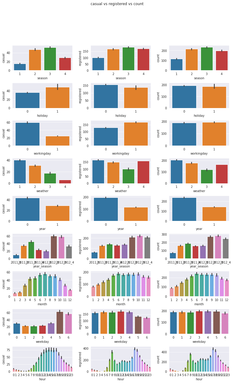
plt.suptitle('casual vs registered vs count')
plt.subplots_adjust(hspace = 0.5, wspace = 0.3)
col_list = ["season","holiday","workingday","weather","year","year_season","month","weekday","hour"]
count_list = ["casual","registered","count"]

for i, col in enumerate(col_list):
    for j, con in enumerate(count_list):
        plt.subplot(9,3,3*i+j+1)
        sns.barplot(train[col],train[con])

In count of holiday, workingday and weekday, there is no difference depending on categories. but in registered and casual, it depend of the categories. So need to look at this part differently.

see relationship between weekday and each count by workingday and holiday

1
2
3
4
5


plt.figure(figsize=(15,6))
plt.subplot(121)
sns.barplot(x="weekday", y="casual", hue="workingday", data=train)
plt.subplot(122)
sns.barplot(x="weekday", y="registered", hue="workingday", data=train)

<matplotlib.axes._subplots.AxesSubplot at 0x7fe7b371f940>

There is no holiday in Tuesday and Thursday. And there is differences when Monday, Wednesday, and Friday.

see relationship between hour and each count by workingday and holiday

 1
 2
 3
 4
 5
 6
 7
 8
 9
10


plt.figure(figsize=(18,11))
plt.subplot(221)
sns.pointplot(x="hour", y="casual", hue="workingday", data=train)
plt.subplot(222)
sns.pointplot(x="hour", y="casual", hue="holiday", data=train)
plt.subplot(223)
sns.pointplot(x="hour", y="registered", hue="workingday", data=train)
plt.subplot(224)
sns.pointplot(x="hour", y="registered", hue="holiday", data=train)
# train.pivot_table(index="hour", columns="workingday", aggfunc="size")

<matplotlib.axes._subplots.AxesSubplot at 0x7fe7b995a0b8>

The number of registered and casual according to workingday and holiday show the opposite pattern. And there are differences in the number of registered according to workingday at the closing hour and the office-going hour. So many registered is can be expected to workers.

correlation

1
2


plt.figure(figsize=(11,11))
sns.heatmap(train.corr(),annot=True,cmap="Blues")

temp and atemp have high correlation and register and have too. And windspeed and outcomes have low correlation(<=0.1) See scatterplot of temp and atemp.

1
2
3


for i, df in enumerate([train,test]):
    plt.subplot(1,2,i+1)
    sns.scatterplot(x = 'temp', y = 'atemp',data = df)

png

In train data, there is strange pattern, but not in test. It seems to be haved wrong value in atemp. So based on correlation and scatterplot, judged to remove atemp

Based on the above results, make new variable.

 1
 2
 3
 4
 5
 6
 7
 8
 9
10
11
12
13
14
15
16
17


df_list = {"train":None, "test" : None}
for name, df in zip(df_list.keys(),[train, test]):
    df['windspeed'] = np.log(df['windspeed']+1)
    df["weekday_working"] = df["weekday"]*df["workingday"]
    df["weekday_holiday"] = df["weekday"]*df["holiday"]
    df['casual_workhour'] = df[['hour', 'workingday']].apply(lambda x: int(x['workingday'] == 0 and 10 <= x['hour'] <= 19), axis=1)
    df['casual_holi_hour'] = df[['hour', 'holiday']].apply(lambda x: int(x['holiday'] == 1 and 9 <= x['hour'] <= 22), axis=1)
    df['register_workhour'] = df[['hour', 'workingday']].apply(
      lambda x:int((x['workingday'] == 1 and (6 <= x['hour'] <= 8 or 17 <= x['hour'] <= 20))
        or (x['workingday'] == 0 and 10 <= x['hour'] <= 15)), axis=1)
    df['register_holi_hour'] = df[['hour', 'holiday']].apply(
      lambda x:int(x['holiday'] == 0 and (7 <= x['hour'] <= 8 or 17 <= x['hour'] <= 18)), axis=1)
    df.drop('atemp',axis=1,inplace=True)
by_season = train.groupby('year_season')[['count']].median()
by_season.columns = ['count_season']
train1 = train.join(by_season, on='year_season').drop('year_season',axis=1)
test1 = test.join(by_season, on='year_season').drop('year_season',axis=1)

Divide predictors and outcomes. And take logging outcomes to normalize.

1
2
3
4


from sklearn.model_selection import train_test_split
y_list = ["casual","registered","count"]
train_x = train1[[col for col in train1.columns if col not in ['casual','registered', 'count']]]
train_y = np.log(train1[y_list]+1)

Modeling

- 1. lightgbm + cross validation

Use lightgbm model, and use cross-validation to prevent overfitting

 1
 2
 3
 4
 5
 6
 7
 8
 9
10
11
12
13
14
15
16
17
18
19
20
21
22
23
24
25
26
27
28
29
30
31
32


import lightgbm as lgb
from sklearn.model_selection import KFold
from sklearn.metrics import mean_squared_error

folds = KFold(n_splits = 5, shuffle = True, random_state = 123)
rms1,rms2 = [],[]
models1,models2 = [], []
for n_fold, (trn_idx, val_idx) in enumerate(folds.split(train1)) :
    x_train, y_train = train_x.ix[trn_idx], train_y.ix[trn_idx] 
    x_val, y_val = train_x.ix[val_idx], train_y.ix[val_idx]
    
    lgb_param = {'boosting_type':'gbdt',
             'num_leaves': 45,
             'max_depth': 30,
            'learning_rate': 0.01, 
            'bagging_fraction' : 0.9,
            'bagging_freq': 20,
            'colsample_bytree': 0.9,
             'metric': 'rmse',
            'min_child_weight': 1,
            'min_child_samples': 10,
             'zero_as_missing': True,
            'objective': 'regression',
            }
    train_set1 = lgb.Dataset(x_train, y_train["registered"], silent=False)
    valid_set1 = lgb.Dataset(x_val, y_val["registered"], silent=False)
    lgb_model1 = lgb.train(params = lgb_param, train_set = train_set1 , num_boost_round=5000, early_stopping_rounds=100,verbose_eval=500, valid_sets=valid_set1)
    train_set2 = lgb.Dataset(x_train, y_train["casual"], silent=False)
    valid_set2 = lgb.Dataset(x_val, y_val["casual"], silent=False)
    lgb_model2 = lgb.train(params = lgb_param, train_set = train_set2 , num_boost_round=5000, early_stopping_rounds=100,verbose_eval=500, valid_sets=valid_set2)
    models1.append(lgb_model1)
    models2.append(lgb_model2)

Training until validation scores don't improve for 100 rounds
[500]	valid_0's rmse: 0.472853
[1000]	valid_0's rmse: 0.462003
Early stopping, best iteration is:
[1388]	valid_0's rmse: 0.459316

see feature importance

1
2
3
4
5
6


tmp = pd.DataFrame({'Feature': x_train.columns, 'Feature importance': lgb_model1.feature_importance()})
tmp = tmp.sort_values(by='Feature importance',ascending=False)
plt.figure(figsize = (15,15))
plt.title('Features importance',fontsize=14)
s = sns.barplot(x='Feature',y='Feature importance',data=tmp)
s.set_xticklabels(s.get_xticklabels(),rotation=90)

 1
 2
 3
 4
 5
 6
 7
 8
 9
10
11
12


preds = []
for model in models1:
    regi_pred = model.predict(test1)
    preds.append(regi_pred)
fin_casual = np.mean(preds, axis=0)

preds = []
for model in models2:
    casual_pred = model.predict(test1)
    preds.append(casual_pred)
fin_regi = np.mean(preds, axis=0)
count_pred1 = np.exp(fin_casual) + np.exp(fin_regi) - 2

- 3. randomforest and gradientboostingregressor

 1
 2
 3
 4
 5
 6
 7
 8
 9
10
11
12
13
14
15
16
17
18
19
20
21
22


from sklearn.ensemble import RandomForestRegressor, GradientBoostingRegressor
preds = {}
regs = {"gbdt": GradientBoostingRegressor(random_state=0),
        "rf": RandomForestRegressor(random_state=0, n_jobs=-1)}
for name, reg in regs.items():
    if name == 'gbdt':
        reg.set_params(n_estimators=1500, min_samples_leaf=6)
    elif name == 'rf':
        reg.set_params(n_estimators=1500, min_samples_leaf=2)
    reg.fit(train_x, train_y['casual'])
    pred_casual = reg.predict(test1)
    pred_casual = np.exp(pred_casual) - 1
    pred_casual[pred_casual < 0] = 0
    if name == 'gbdt':
        reg.set_params(n_estimators=1500, min_samples_leaf=6)
    elif name == 'rf':
        reg.set_params(n_estimators=1500, min_samples_leaf=2)
    reg.fit(train_x, train_y['registered'])
    pred_registered = reg.predict(test1)
    pred_registered = np.exp(pred_registered) - 1
    pred_registered[pred_registered < 0] = 0
    preds[name] = pred_casual + pred_registered

1
2
3
4
5
6


tmp = pd.DataFrame({'Feature': x_train.columns, 'Feature importance': reg.feature_importances_})
tmp = tmp.sort_values(by='Feature importance',ascending=False)
plt.figure(figsize = (15,15))
plt.title('Features importance',fontsize=14)
s = sns.barplot(x='Feature',y='Feature importance',data=tmp)
s.set_xticklabels(s.get_xticklabels(),rotation=90)

1
2
3
4


pred_mean = (count_pred1 + count_pred2 + preds['gbdt'] + preds['rf'])/4
sample = pd.read_csv("../input/bike-sharing-demand/sampleSubmission.csv")
sample["count"] = pred_mean
sample.to_csv("sample.csv",index=False)

Result rmsle is 0.38081

자전거 수요 예측