 1
 2
 3
 4
 5
 6
 7
 8
 9
10
11
12
|
import pandas as pd
import numpy as np
import matplotlib.pyplot as plt
import seaborn as sns
from scipy import stats
import statsmodels.api as sm
from sklearn.model_selection import train_test_split
from sklearn.metrics import mean_squared_error
plt.style.use('fivethirtyeight')

sales = pd.read_csv('Album_sales_2.txt',sep='\t')
sales
|
|
adverts |
sales |
airplay |
attract |
| 0 |
10.256 |
330 |
43 |
10 |
| 1 |
985.685 |
120 |
28 |
7 |
| 2 |
1445.563 |
360 |
35 |
7 |
| 3 |
1188.193 |
270 |
33 |
7 |
| 4 |
574.513 |
220 |
44 |
5 |
| ... |
... |
... |
... |
... |
| 195 |
910.851 |
190 |
26 |
7 |
| 196 |
888.569 |
240 |
14 |
6 |
| 197 |
800.615 |
250 |
34 |
6 |
| 198 |
1500.000 |
230 |
11 |
8 |
| 199 |
785.694 |
110 |
20 |
9 |
- advers : 광고비
- sales: 판매량
- airplay : 음반 출시전 한 주 동안 노래들이 라디오1에 방송된 횟수
- attract : 밴드 매력(0~10)
1. EDA
<class 'pandas.core.frame.DataFrame'>
RangeIndex: 200 entries, 0 to 199
Data columns (total 4 columns):
 #   Column   Non-Null Count  Dtype
---  ------   --------------  -----
 0   adverts  200 non-null    float64
 1   sales    200 non-null    int64
 2   airplay  200 non-null    int64
 3   attract  200 non-null    int64
dtypes: float64(1), int64(3)
memory usage: 6.4 KB
|
adverts |
sales |
airplay |
attract |
| count |
200.000000 |
200.000000 |
200.000000 |
200.00000 |
| mean |
614.412255 |
193.200000 |
27.500000 |
6.77000 |
| std |
485.655208 |
80.698957 |
12.269585 |
1.39529 |
| min |
9.104000 |
10.000000 |
0.000000 |
1.00000 |
| 25% |
215.917750 |
137.500000 |
19.750000 |
6.00000 |
| 50% |
531.916000 |
200.000000 |
28.000000 |
7.00000 |
| 75% |
911.225500 |
250.000000 |
36.000000 |
8.00000 |
| max |
2271.860000 |
360.000000 |
63.000000 |
10.00000 |
1
2
3
4
5
|
plt.style.use('seaborn-pastel')
plt.figure(figsize=(10,10))
for i,j in enumerate(sales.columns):
    plt.subplot(2,2,i+1)
    sns.histplot(sales[j])
|

<seaborn.axisgrid.PairGrid at 0x1e5f655a940>

1
|
sns.heatmap(sales.corr(),annot=True,cmap='Blues')
|
<AxesSubplot:>

`시각화를 통해 보았을 때 advert가 치우쳐서 변수 변환이 필요할 수 있다는 점 빼고 큰 특징은 보이지 않는다.
상관성이 좀 있는 편인데 일단 회귀 분석을 진행하면서 결과를 살펴봐야겠다.
2. train, test로 분리 후 다중회귀분석 결과 해석
1
|
x_train, x_test, y_train, y_test = train_test_split(sales.iloc[:,[0,2,3]], sales['sales'],)
|
상수항 넣었을 때
1
|
x_data = sm.add_constant(x_train, has_constant = "add")
|
1
2
3
4
|
# const넣음
model = sm.OLS(y_train,x_data)
result = model.fit()
result.summary()
|
OLS Regression Results
| Dep. Variable: | sales | R-squared: | 0.651 |
| Model: | OLS | Adj. R-squared: | 0.644 |
| Method: | Least Squares | F-statistic: | 90.71 |
| Date: | Fri, 09 Oct 2020 | Prob (F-statistic): | 3.44e-33 |
| Time: | 14:24:41 | Log-Likelihood: | -789.91 |
| No. Observations: | 150 | AIC: | 1588. |
| Df Residuals: | 146 | BIC: | 1600. |
| Df Model: | 3 | | |
| Covariance Type: | nonrobust | | |
| coef | std err | t | P>|t| | [0.025 | 0.975] |
| const | -36.6149 | 21.619 | -1.694 | 0.092 | -79.341 | 6.111 |
| adverts | 0.0825 | 0.008 | 10.032 | 0.000 | 0.066 | 0.099 |
| airplay | 3.4240 | 0.314 | 10.897 | 0.000 | 2.803 | 4.045 |
| attract | 12.5468 | 2.997 | 4.187 | 0.000 | 6.624 | 18.470 |
| Omnibus: | 0.238 | Durbin-Watson: | 1.725 |
| Prob(Omnibus): | 0.888 | Jarque-Bera (JB): | 0.189 |
| Skew: | 0.086 | Prob(JB): | 0.910 |
| Kurtosis: | 2.972 | Cond. No. | 4.41e+03 |
1
2
|
y_pred = result.predict(ols.add_constant(x_test, has_constant = "add"))
mean_squared_error(y_pred,y_test)
|
2128.1345418881824
1
2
3
4
|
# 안 넣음
model2 = sm.OLS(y_train,x_train)
result2 = model2.fit()
result2.summary()
|
OLS Regression Results
| Dep. Variable: | sales | R-squared (uncentered): | 0.950 |
| Model: | OLS | Adj. R-squared (uncentered): | 0.949 |
| Method: | Least Squares | F-statistic: | 928.3 |
| Date: | Sun, 11 Oct 2020 | Prob (F-statistic): | 2.75e-95 |
| Time: | 23:09:26 | Log-Likelihood: | -791.37 |
| No. Observations: | 150 | AIC: | 1589. |
| Df Residuals: | 147 | BIC: | 1598. |
| Df Model: | 3 | | |
| Covariance Type: | nonrobust | | |
| coef | std err | t | P>|t| | [0.025 | 0.975] |
| adverts | 0.0797 | 0.008 | 9.830 | 0.000 | 0.064 | 0.096 |
| airplay | 3.3006 | 0.308 | 10.731 | 0.000 | 2.693 | 3.908 |
| attract | 8.1136 | 1.468 | 5.525 | 0.000 | 5.212 | 11.016 |
| Omnibus: | 0.694 | Durbin-Watson: | 1.762 |
| Prob(Omnibus): | 0.707 | Jarque-Bera (JB): | 0.587 |
| Skew: | 0.153 | Prob(JB): | 0.745 |
| Kurtosis: | 2.990 | Cond. No. | 300. |
aic는 비슷하나 R-squared 면에서 상수항이 없는게 나음
1
2
|
y_pred = result2.predict(x_test)
mean_squared_error(y_pred,y_test)
|
2093.0726936877363
1
2
|
plt.plot(y_test.values)
plt.plot(y_pred.values)
|

VIF
1
2
|
from statsmodels.stats.outliers_influence import variance_inflation_factor
[variance_inflation_factor(x_train.values,i) for i in range(3)]
|
[2.6632477766856404, 5.761240629832455, 6.855611086457372]
대체로 크게 나오는 편은 아니다.
변수가 적어 모든 변수 조합에서 Variance와 mse를 살펴 봄
1
2
3
4
5
6
|
from itertools import combinations
joint = []
for i in range(1,4):
    k = combinations(x_train.columns,i)
    for j in k:
        joint.append(j)
|
[('adverts',),
 ('airplay',),
 ('attract',),
 ('adverts', 'airplay'),
 ('adverts', 'attract'),
 ('airplay', 'attract'),
 ('adverts', 'airplay', 'attract')]
1
2
3
4
5
6
|
stepw = []
for i in joint:
    model = sm.OLS(y_train,x_train[list(i)])
    result = model.fit()
    y_pred = result.predict(x_test[list(i)])
    stepw.append([list(i),result.aic,mean_squared_error(y_pred,y_test)])
|
1
2
3
|
stepw_frame = pd.DataFrame(stepw, columns=['Variables','AIC','MSE'])
stepw_frame.set_index('Variables',inplace=True)
stepw_frame
|
|
AIC |
MSE |
| Variables |
|
|
| [adverts] |
1832.620857 |
9775.286334 |
| [airplay] |
1716.242475 |
5246.164309 |
| [attract] |
1727.874967 |
6423.816111 |
| [adverts, airplay] |
1615.042139 |
2447.023190 |
| [adverts, attract] |
1673.510244 |
3376.763066 |
| [airplay, attract] |
1662.523096 |
4237.857648 |
| [adverts, airplay, attract] |
1588.737818 |
2093.072694 |
3개 다 선택했을 때 값이 가장 적게 나온다.
다중회귀분석의 매개변수별 신뢰구간
|
0 |
1 |
| adverts |
0.063717 |
0.095782 |
| airplay |
2.692710 |
3.908404 |
| attract |
5.211536 |
11.015580 |
3. 독립성, 정규성 가정 평가
1
2
|
# 독립성
sns.regplot(result2.fittedvalues, result2.resid, lowess=True, line_kws={'color': 'red'})
|

1
2
|
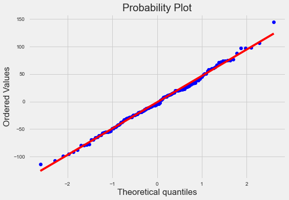
#정규성
stats.probplot(result2.resid,plot=plt);
|
1
|
stats.shapiro(result2.resid)
|
(0.9950959086418152, 0.8982971906661987)
- 독립성과 정규성을 만족하는 편이다.
- summary에서 durbin-watson 값이 1.5~2.5 안에 있어야 정상이라고 함
4. 표준화잔차, cook’s distance, DFBeta, 공분산비 보기
- 표준화잔차(standard_resid) : 잔차를 표준오차로 나눈 값
- cook’s distance : 관측치가 제거되었을 때 모수 추정값들의 (동시적) 변화량 척도
- DFBeta : 관측값이 각각의 회귀계수에 미치는 영향력을 측정
- DFFITS : 관측치가 예측값에서 보유하고 있는 영향력을 측정
1
2
3
|
infl = result2.get_influence()
sm_fr = infl.summary_frame()
sm_fr
|
|
dfb_adverts |
dfb_airplay |
dfb_attract |
cooks_d |
standard_resid |
hat_diag |
dffits_internal |
student_resid |
dffits |
| 23 |
-0.000441 |
-0.009346 |
0.000516 |
0.000159 |
-0.238252 |
0.008315 |
-0.021816 |
-0.237486 |
-0.021746 |
| 33 |
-0.005728 |
0.022027 |
-0.020366 |
0.000221 |
-0.152693 |
0.027656 |
-0.025751 |
-0.152185 |
-0.025666 |
| 117 |
-0.004076 |
0.000292 |
-0.001237 |
0.000026 |
-0.133886 |
0.004372 |
-0.008872 |
-0.133438 |
-0.008842 |
| 93 |
-0.054948 |
-0.212492 |
0.243871 |
0.020558 |
1.247608 |
0.038112 |
0.248342 |
1.249992 |
0.248816 |
| 64 |
-0.029928 |
-0.040401 |
0.068245 |
0.001846 |
0.489364 |
0.022606 |
0.074423 |
0.488095 |
0.074230 |
| ... |
... |
... |
... |
... |
... |
... |
... |
... |
... |
| 153 |
-0.050052 |
0.055071 |
-0.006892 |
0.002166 |
0.452345 |
0.030779 |
0.080610 |
0.451118 |
0.080391 |
| 130 |
0.002361 |
0.053852 |
-0.030313 |
0.001554 |
0.697670 |
0.009485 |
0.068270 |
0.696447 |
0.068151 |
| 104 |
-0.048983 |
0.167837 |
-0.092858 |
0.010958 |
0.829723 |
0.045577 |
0.181316 |
0.828839 |
0.181123 |
| 161 |
0.094157 |
0.025861 |
-0.098308 |
0.005490 |
-1.127330 |
0.012794 |
-0.128339 |
-1.128377 |
-0.128458 |
| 183 |
-0.028555 |
-0.003881 |
0.015144 |
0.000299 |
-0.089645 |
0.100417 |
-0.029951 |
-0.089342 |
-0.029850 |
1
2
3
4
5
6
7
|
album_sales_diagnostics = pd.concat([x_train,y_train],axis=1)

album_sales_diagnostics['cook'] = infl.cooks_distance[0]
album_sales_diagnostics['resid_std'] = infl.resid_studentized
album_sales_diagnostics[['dfbeta_adverts','dfbeta_airplay','dfbeta_attract']] = infl.dfbeta
album_sales_diagnostics['covariance'] = infl.cov_ratio
album_sales_diagnostics.head()
|
|
adverts |
airplay |
attract |
sales |
cook |
resid_std |
dfbeta_adverts |
dfbeta_airplay |
dfbeta_attract |
covariance |
| 23 |
656.137 |
34 |
7 |
210 |
0.000159 |
-0.238252 |
-0.000004 |
-0.002884 |
0.000760 |
1.028055 |
| 33 |
759.862 |
6 |
7 |
130 |
0.000221 |
-0.152693 |
-0.000047 |
0.006798 |
-0.030006 |
1.049221 |
| 117 |
624.538 |
20 |
5 |
150 |
0.000026 |
-0.133886 |
-0.000033 |
0.000090 |
-0.001823 |
1.024796 |
| 93 |
268.598 |
1 |
7 |
140 |
0.020558 |
1.247608 |
-0.000445 |
-0.065233 |
0.357433 |
1.027779 |
| 64 |
391.749 |
22 |
9 |
200 |
0.001846 |
0.489364 |
-0.000243 |
-0.012459 |
0.100476 |
1.039201 |
영향력이 큰 사례
cook distance가 큰 순서대로 정렬
- 4/표본수 이상이면 영향력이 크다고 할 수 있음.
1
2
|
album.resid_std = np.abs(album.resid_std)
album.sort_values(by = ['cook','resid_std'],ascending=[False, False])
|
|
adverts |
airplay |
attract |
sales |
cook |
resid_std |
dfbeta_adverts |
dfbeta_airplay |
dfbeta_attract |
covariance |
| 168 |
145.585 |
42 |
8 |
360 |
0.075704 |
3.067079 |
-0.002579 |
0.071664 |
0.107867 |
0.857218 |
| 0 |
10.256 |
43 |
10 |
330 |
0.065682 |
2.262619 |
-0.002828 |
0.025215 |
0.302940 |
0.953043 |
| 118 |
912.349 |
57 |
6 |
230 |
0.053361 |
1.709781 |
-0.000618 |
-0.111819 |
0.430083 |
1.013622 |
| 99 |
1000.000 |
5 |
7 |
250 |
0.050402 |
2.064131 |
0.001338 |
-0.098943 |
0.371103 |
0.967650 |
| 54 |
1542.329 |
33 |
8 |
190 |
0.050391 |
2.267631 |
-0.002619 |
0.004308 |
0.094568 |
0.944246 |
| ... |
... |
... |
... |
... |
... |
... |
... |
... |
... |
... |
| 79 |
15.313 |
22 |
5 |
110 |
0.000026 |
0.092506 |
0.000056 |
-0.000595 |
-0.005664 |
1.029915 |
| 117 |
624.538 |
20 |
5 |
150 |
0.000026 |
0.133886 |
-0.000033 |
0.000090 |
-0.001823 |
1.024796 |
| 179 |
26.598 |
47 |
8 |
220 |
0.000025 |
0.045893 |
0.000048 |
-0.001569 |
-0.000459 |
1.056691 |
| 141 |
893.355 |
26 |
6 |
210 |
0.000023 |
0.089516 |
0.000044 |
0.000217 |
-0.001188 |
1.029495 |
| 109 |
102.568 |
22 |
7 |
140 |
0.000013 |
0.050878 |
-0.000035 |
-0.000455 |
0.007294 |
1.036476 |
데이터 출처 : SpringSchool