2-1-1 : 코로나 인구대비 확진자수가 많은 상위 5개국 누적확진자수, 일일확진자수, 누적사망자수, 일일사망자수 선그래프로 시각화
2-1-2 : 코로나 검사자수, 확진자수, 완치자수, 사망자수, 인구수를 바탕으로 위험지수를 만들고 그 지수를 바탕으로 국가별 위험도를 판단, 상위 10개국에 대해 위험지수 막대그래프로 시각화
2-1-3 : 한국 누적 확진자수를 바탕으로 시계열 예측. 선형 시계열과 비선형 시계열 2가지로 모델링하고 평가. 5월 16일 이후 데이터로 테스트.
1
2
3
4
5
6
7
8
import numpy as np
import pandas as pd
import seaborn as sns
import matplotlib.pyplot as plt
% matplotlib inline
import statsmodels.api as sm
from statsmodels.graphics.tsaplots import plot_acf , plot_pacf
from statsmodels.tsa.seasonal import seasonal_decompose
1
2
corona = pd . read_csv ( '../data/covid_19_data.csv' , index_col = 'ObservationDate' , parse_dates = True )
corona . info ()
<class 'pandas.core.frame.DataFrame'>
DatetimeIndex: 109382 entries, 2020-01-22 to 2020-09-13
Data columns (total 7 columns):
 #   Column          Non-Null Count   Dtype
---  ------          --------------   -----
 0   SNo             109382 non-null  int64
 1   Province/State  75709 non-null   object
 2   Country/Region  109382 non-null  object
 3   Last Update     109382 non-null  object
 4   Confirmed       109382 non-null  float64
 5   Deaths          109382 non-null  float64
 6   Recovered       109382 non-null  float64
dtypes: float64(3), int64(1), object(3)
memory usage: 6.7+ MB
SNo
Province/State
Country/Region
Last Update
Confirmed
Deaths
Recovered
ObservationDate
2020-01-22
1
Anhui
Mainland China
1/22/2020 17:00
1.0
0.0
0.0
2020-01-22
2
Beijing
Mainland China
1/22/2020 17:00
14.0
0.0
0.0
2020-01-22
3
Chongqing
Mainland China
1/22/2020 17:00
6.0
0.0
0.0
2020-01-22
4
Fujian
Mainland China
1/22/2020 17:00
1.0
0.0
0.0
2020-01-22
5
Gansu
Mainland China
1/22/2020 17:00
0.0
0.0
0.0
2-1-1 DatetimeIndex(['2020-01-22', '2020-01-23', '2020-01-24', '2020-01-25',
'2020-01-26', '2020-01-27', '2020-01-28', '2020-01-29',
'2020-01-30', '2020-01-31',
...
'2020-09-04', '2020-09-05', '2020-09-06', '2020-09-07',
'2020-09-08', '2020-09-09', '2020-09-10', '2020-09-11',
'2020-09-12', '2020-09-13'],
dtype='datetime64[ns]', name='ObservationDate', length=236, freq=None)
1
2
3
last_day = corona . loc [ corona . index == '2020-09-13' ]
last_day_country = last_day . groupby ( 'Country/Region' )[[ 'Confirmed' , 'Deaths' , 'Recovered' ]] . sum ()
last_day_country
Confirmed
Deaths
Recovered
Country/Region
Afghanistan
38716.0
1420.0
31638.0
Albania
11353.0
334.0
6569.0
Algeria
48254.0
1612.0
34037.0
Andorra
1344.0
53.0
943.0
Angola
3388.0
134.0
1301.0
...
...
...
...
West Bank and Gaza
30574.0
221.0
20082.0
Western Sahara
10.0
1.0
8.0
Yemen
2011.0
583.0
1212.0
Zambia
13539.0
312.0
12260.0
Zimbabwe
7526.0
224.0
5678.0
1
2
3
Confirmed_list = last_day_country . sort_values ( by = 'Confirmed' , ascending = False )[: 5 ] . index
Deaths_list = last_day_country . sort_values ( by = 'Deaths' , ascending = False )[: 5 ] . index
last_day_country . sort_values ( by = 'Confirmed' , ascending = False )
Confirmed
Deaths
Recovered
Country/Region
US
6519573.0
194071.0
2451406.0
India
4754356.0
78586.0
3702595.0
Brazil
4330455.0
131625.0
3723206.0
Russia
1059024.0
18517.0
873684.0
Peru
722832.0
30526.0
559321.0
...
...
...
...
Laos
23.0
0.0
21.0
Saint Kitts and Nevis
17.0
0.0
17.0
Holy See
12.0
0.0
12.0
Western Sahara
10.0
1.0
8.0
MS Zaandam
9.0
2.0
0.0
Index(['US', 'India', 'Brazil', 'Russia', 'Peru'], dtype='object', name='Country/Region')
1
2
Top_Confrimed = corona . loc [ corona [ 'Country/Region' ] . isin ( Confirmed_list )]
Top_Deaths = corona . loc [ corona [ 'Country/Region' ] . isin ( Deaths_list )]
1
2
five_top_Confirmed = Top_Confrimed . groupby ([ 'Country/Region' , 'ObservationDate' ])[ 'Confirmed' ] . sum ()
five_top_Deaths = Top_Deaths . groupby ([ 'Country/Region' , 'ObservationDate' ])[ 'Deaths' ] . sum ()
1
2
five_top_Confirmed . unstack ( 'Country/Region' ) . plot ()
five_top_Deaths . unstack ( 'Country/Region' ) . plot ()
1
2
3
4
f_u = five_top_Confirmed . unstack ( 'Country/Region' )
f_d = five_top_Deaths . unstack ( 'Country/Region' )
one_day_Confirmed = f_u - f_u . shift ( 1 )
one_day_Deaths = f_d - f_d . shift ( 1 )
Country/Region
Brazil
India
Peru
Russia
US
ObservationDate
2020-01-22
NaN
NaN
NaN
NaN
NaN
2020-01-23
NaN
NaN
NaN
NaN
0.0
2020-01-24
NaN
NaN
NaN
NaN
1.0
2020-01-25
NaN
NaN
NaN
NaN
0.0
2020-01-26
NaN
NaN
NaN
NaN
3.0
...
...
...
...
...
...
2020-09-09
35816.0
95735.0
4615.0
5172.0
34256.0
2020-09-10
40557.0
96551.0
6586.0
5310.0
35286.0
2020-09-11
43718.0
97570.0
7291.0
5421.0
47192.0
2020-09-12
33523.0
94372.0
6603.0
5406.0
41471.0
2020-09-13
14768.0
0.0
6162.0
5361.0
34359.0
1
2
3
one_day_Confirmed . fillna ( 0 ) . plot ()
one_day_Deaths . fillna ( 0 ) . plot ()
plt . ylim ( - 100 , 5000 )
(-100.0, 5000.0)
2-1-2
risk = (확진자 수 - 사망자 수 - 완치자 수)/(state * 10000)
국가별 1달 risk 계산 평균 -> top 10
1
2
3
one_month = corona [ '2020-08-14' :]
a = one_month . groupby ([ 'ObservationDate' , 'Country/Region' ])[[ 'Confirmed' , 'Deaths' , 'Recovered' ]] . sum ()
a
Confirmed
Deaths
Recovered
ObservationDate
Country/Region
2020-08-14
Afghanistan
37431.0
1363.0
26714.0
Albania
7117.0
219.0
3695.0
Algeria
37664.0
1351.0
26308.0
Andorra
989.0
53.0
863.0
Angola
1852.0
86.0
584.0
...
...
...
...
...
2020-09-13
West Bank and Gaza
30574.0
221.0
20082.0
Western Sahara
10.0
1.0
8.0
Yemen
2011.0
583.0
1212.0
Zambia
13539.0
312.0
12260.0
Zimbabwe
7526.0
224.0
5678.0
ObservationDate
Confirmed
Deaths
Recovered
Country/Region
Afghanistan
2020-08-14
37431.0
1363.0
26714.0
Albania
2020-08-14
7117.0
219.0
3695.0
Algeria
2020-08-14
37664.0
1351.0
26308.0
Andorra
2020-08-14
989.0
53.0
863.0
Angola
2020-08-14
1852.0
86.0
584.0
...
...
...
...
...
West Bank and Gaza
2020-09-13
30574.0
221.0
20082.0
Western Sahara
2020-09-13
10.0
1.0
8.0
Yemen
2020-09-13
2011.0
583.0
1212.0
Zambia
2020-09-13
13539.0
312.0
12260.0
Zimbabwe
2020-09-13
7526.0
224.0
5678.0
1
2
3
b = last_day . groupby ( 'Country/Region' )[ 'SNo' ] . count ()
b . name = 'State_Num'
b . sort_values ( ascending = False )[: 10 ]
Country/Region
Russia            83
US                58
Japan             49
India             37
Colombia          33
Mexico            32
Mainland China    31
Ukraine           27
Brazil            27
Peru              26
Name: State_Num, dtype: int64
1
df = a . reset_index ( level = 0 ) . join ( b , how = 'left' )
1
df . set_index ( 'ObservationDate' , append = True , inplace = True )
Confirmed
Deaths
Recovered
State_Num
Country/Region
ObservationDate
Afghanistan
2020-08-14
37431.0
1363.0
26714.0
1
2020-08-15
37551.0
1370.0
27166.0
1
2020-08-16
37596.0
1375.0
27166.0
1
2020-08-17
37599.0
1375.0
27166.0
1
2020-08-18
37599.0
1375.0
27166.0
1
...
...
...
...
...
...
Zimbabwe
2020-09-09
7429.0
222.0
5542.0
1
2020-09-10
7453.0
222.0
5635.0
1
2020-09-11
7479.0
224.0
5660.0
1
2020-09-12
7508.0
224.0
5675.0
1
2020-09-13
7526.0
224.0
5678.0
1
1
2
df [ 'risk_pi' ] = ( df [ 'Confirmed' ] - df [ 'Deaths' ] - df [ 'Recovered' ]) / ( df [ 'State_Num' ] * 10000 )
df . head ()
Confirmed
Deaths
Recovered
State_Num
risk_pi
Country/Region
ObservationDate
Afghanistan
2020-08-14
37431.0
1363.0
26714.0
1
0.9354
2020-08-15
37551.0
1370.0
27166.0
1
0.9015
2020-08-16
37596.0
1375.0
27166.0
1
0.9055
2020-08-17
37599.0
1375.0
27166.0
1
0.9058
2020-08-18
37599.0
1375.0
27166.0
1
0.9058
1
2
3
4
5
# last_day_country['risk_pi'] = (last_day_country['Confirmed']/1000000 - last_day_country['Recovered']/1000000)/1000000
# top_risk_list = last_day_country.sort_values(by='risk_pi',ascending=False)[:10]
df_risk = df . groupby ( 'Country/Region' )[ 'risk_pi' ] . mean ()
top_risk_list = df_risk . sort_values ( ascending = False )[: 10 ]
top_risk_list
Country/Region
Bangladesh      10.533694
Argentina       10.164006
South Africa     7.527106
US               6.239020
Philippines      6.162177
Belgium          5.627332
Iraq             5.155116
Bolivia          5.124435
Honduras         4.621997
Romania          4.466106
Name: risk_pi, dtype: float64
1
top_risk_list . plot . bar ()
<AxesSubplot:xlabel='Country/Region'>
2-1-3
1
2
3
k_c = corona [ corona [ 'Country/Region' ] == 'South Korea' ]
print ( len ( k_c ))
print ( len ( k_c . index . unique ()))
236
236
1
from statsmodels.tsa.stattools import adfuller # 정상성 판별 여부
1
2
3
k = k_c [ 'Confirmed' ]
korea_co = ( k - k . shift ( 1 )) . dropna ()
korea_co . plot ()
<AxesSubplot:xlabel='ObservationDate'>
1
2
train = korea_co [: '2020-05-15' ]
test = korea_co [ '2020-05-16' : '2020-06-15' ]
(-2.692880412737049,
 0.07527839224613403,
 5,
 108,
 {'1%': -3.4924012594942333,
  '5%': -2.8886968193364835,
  '10%': -2.5812552709190673},
 1147.051801657943)
` 1차 차분
1
2
diff1 = ( train - train . shift ( 1 )) . dropna ()
adfuller ( diff1 )
(-5.228238034317768,
 7.697004182819284e-06,
 2,
 110,
 {'1%': -3.4912451337340342,
  '5%': -2.8881954545454547,
  '10%': -2.5809876033057852},
 1139.877102390829)
1
2
3
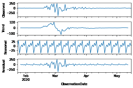
decomposition = seasonal_decompose ( diff1 )
decomposition . plot ()
plt . show ()
1
2
diff2 = ( diff1 - diff1 . shift ( 1 )) . dropna ()
adfuller ( diff2 )
(-6.291128356594684,
 3.5970963612700875e-08,
 6,
 105,
 {'1%': -3.4942202045135513,
  '5%': -2.889485291005291,
  '10%': -2.5816762131519275},
 1140.9946617995597)
2차 차분
1
2
3
decomposition = seasonal_decompose ( diff2 )
decomposition . plot ()
plt . show ()
1
2
plot_acf ( diff1 );
plot_pacf ( diff1 );
1
2
model = sm . tsa . statespace . SARIMAX ( train ,
order = [ 1 , 1 , 1 ], trend = 't' )
C:\Users\Gyu\Anaconda3\envs\py37\lib\site-packages\statsmodels\tsa\base\tsa_model.py:165: ValueWarning: No frequency information was provided, so inferred frequency D will be used.
  % freq, ValueWarning)
1
2
result = model . fit ()
result . summary ()
Statespace Model Results
Dep. Variable: Confirmed No. Observations: 114
Model: SARIMAX(1, 1, 1) Log Likelihood -641.888
Date: Sun, 27 Sep 2020 AIC 1291.777
Time: 10:40:43 BIC 1302.687
Sample: 01-23-2020 HQIC 1296.204
- 05-15-2020
Covariance Type: opg
coef std err z P>|z| [0.025 0.975]
drift -0.0210 0.162 -0.129 0.897 -0.339 0.297
ar.L1 -0.1768 0.215 -0.821 0.412 -0.599 0.245
ma.L1 -0.0869 0.199 -0.437 0.662 -0.476 0.302
sigma2 5025.8920 309.739 16.226 0.000 4418.815 5632.969
Ljung-Box (Q): 34.23 Jarque-Bera (JB): 350.68
Prob(Q): 0.73 Prob(JB): 0.00
Heteroskedasticity (H): 0.01 Skew: -0.03
Prob(H) (two-sided): 0.00 Kurtosis: 11.63
Warnings:
[1] Covariance matrix calculated using the outer product of gradients (complex-step).
1
pred = result . predict ( start = '2020-05-16' , end = '2020-06-15' )
1
2
3
train . plot ( label = 'Train' )
test . plot ( label = 'Test' )
pred . plot ( label = 'pred' )
<AxesSubplot:xlabel='ObservationDate'>
1
2
from sklearn.metrics import mean_squared_error
mean_squared_error ( test , pred )
3631.3045190567364
1
2
3
4
model = sm . tsa . statespace . SARIMAX ( train ,
order = [ 1 , 1 , 1 ], trend = [ 0 , 1 , 1 ])
result = model . fit ()
result . summary ()
C:\Users\Gyu\Anaconda3\envs\py37\lib\site-packages\statsmodels\tsa\base\tsa_model.py:165: ValueWarning: No frequency information was provided, so inferred frequency D will be used.
  % freq, ValueWarning)
Statespace Model Results
Dep. Variable: Confirmed No. Observations: 114
Model: SARIMAX(1, 1, 1) Log Likelihood -641.925
Date: Sun, 27 Sep 2020 AIC 1293.851
Time: 10:42:26 BIC 1307.488
Sample: 01-23-2020 HQIC 1299.384
- 05-15-2020
Covariance Type: opg
coef std err z P>|z| [0.025 0.975]
drift -0.0008 0.735 -0.001 0.999 -1.441 1.439
trend.2 -0.0002 0.016 -0.015 0.988 -0.031 0.031
ar.L1 -0.1758 0.224 -0.785 0.433 -0.615 0.263
ma.L1 -0.0878 0.207 -0.425 0.671 -0.493 0.317
sigma2 5216.6180 347.385 15.017 0.000 4535.756 5897.480
Ljung-Box (Q): 34.24 Jarque-Bera (JB): 350.89
Prob(Q): 0.73 Prob(JB): 0.00
Heteroskedasticity (H): 0.01 Skew: -0.04
Prob(H) (two-sided): 0.00 Kurtosis: 11.63
Warnings:
[1] Covariance matrix calculated using the outer product of gradients (complex-step).
1
2
3
4
pred = result . predict ( start = '2020-05-16' , end = '2020-06-15' )
train . plot ( label = 'Train' )
test . plot ( label = 'Test' )
pred . plot ( label = 'pred' )
<AxesSubplot:xlabel='ObservationDate'>
1
mean_squared_error ( test , pred )
6478.176590606611
1
2
3
4
from statsmodels.tsa.api import ExponentialSmoothing
model = ExponentialSmoothing ( np . asarray ( train ),
trend = 'add' )
model_result = model . fit ()
ExponentialSmoothing Model Results
Dep. Variable: endog No. Observations: 114
Model: ExponentialSmoothing SSE 571027.819
Optimized: True AIC 979.165
Trend: Additive BIC 990.110
Seasonal: None AICC 979.950
Seasonal Periods: None Date: Sun, 27 Sep 2020
Box-Cox: False Time: 10:46:34
Box-Cox Coeff.: None
coeff code optimized
smoothing_level 0.7647937 alpha True
smoothing_slope 0.000000 beta True
initial_level 0.000000 l.0 True
initial_slope 0.1845664 b.0 True
1
2
3
y_hat = pd . DataFrame ( test . copy ())
y_hat [ 'ES' ] = model_result . forecast ( len ( test ))
mean_squared_error ( y_hat [ 'Confirmed' ], y_hat [ 'ES' ])
360.9693621017652
1
2
3
4
train . plot ( label = 'Train' )
test . plot ( label = 'Test' )
y_hat [ 'ES' ] . plot ( label = 'ES' )
plt . legend ()
1
2
3
model = ExponentialSmoothing ( np . asarray ( train + 1 ), trend = 'mul' )
model_result = model . fit ()
model_result . summary ()
ExponentialSmoothing Model Results
Dep. Variable: endog No. Observations: 114
Model: ExponentialSmoothing SSE 559193.862
Optimized: True AIC 976.778
Trend: Multiplicative BIC 987.723
Seasonal: None AICC 977.563
Seasonal Periods: None Date: Sun, 27 Sep 2020
Box-Cox: False Time: 10:47:32
Box-Cox Coeff.: None
coeff code optimized
smoothing_level 0.7749651 alpha True
smoothing_slope 0.000000 beta True
initial_level 0.4787151 l.0 True
initial_slope 0.9574234 b.0 True
1
2
3
y_hat = pd . DataFrame ( test . copy ())
y_hat [ 'ES' ] = model_result . forecast ( len ( test ))
mean_squared_error ( y_hat [ 'Confirmed' ], y_hat [ 'ES' ])
995.7063961726025
1
2
3
4
train . plot ( label = 'Train' )
test . plot ( label = 'Test' )
y_hat [ 'ES' ] . plot ( label = 'ES' )
plt . legend ()
<matplotlib.legend.Legend at 0x2212c6de470>